Introduction
Qbox is a First-Principles Molecular Dynamics code. It can be used to compute the electronic structure of atoms, molecules, solids and liquids within the Density Functional Theory (DFT) formalism. It can also be used to perform first-principles molecular dynamics (FPMD) simulations using forces computed within DFT. Qbox computes the solutions of the Kohn-Sham equations using a plane wave basis set and norm-conserving pseudopotentials. Notable Qbox features include:
DFT-GGA and hybrid DFT electronic structure
Born-Oppenheimer and Car-Parrinello molecular dynamics
NVT simulations with stochastic thermostats
NPT simulations
Constrained simulations and thermodynamic integration
Maximally localized Wannier functions
Electronic structure in constant electric field
Use as a DFT engine in client-server coupling to other software
Basic Operation
Qbox reads input from standard input and writes output to standard output. It can be used either interactively or in batch mode.
Command line options
A set of command line options can be used
when invoking Qbox to optimize the distribution of computations among MPI tasks.
The -nstb (number of state blocks), -nkpb (number of k-point blocks)
and -nspb (number of spin blocks) command line options are used
to partition MPI tasks into a four-dimensional
communicator of dimensions ngb x nstb x nkpb x nspb. The ngb
value (number of G vector blocks) is inferred from the total number
of tasks and the values of the three other parameters. Slater determinants
(represented by the Fourier coefficients of all states) are
distributed over rectangular process grids of size ngb x nstb.
Slater determinants indexed by different k-points are distributed among
nkpb blocks of size ngb x nstb.
Slater determinants of different spin indices are
distributed among nspb blocks of size ngb x nstb x nkpb.
The dimensions of the communicator are printed on output. For example,
invoking Qbox with a total of 240 tasks and using the following arguments:
$ qb -nstb 2 -nkpb 5 -nspb 2
results in the following output:
MPIdata::comm 12x2x5x2
Slater determinants are represented on rectangular 12x2 process grids. There are 5 such process grids for each of the 2 spin components of the wave functions.
The default value of nstb, nkpb and nspb is 1. The nspb value
can only be 1 or 2.
Interactive mode
In interactive mode, Qbox is started by invoking the executable name:
$ qb
For parallel operation, the executable must be invoked using the mpirun command (shown here for 4 parallel tasks):
$ mpirun -np 4 qb
Qbox first prints information about the code release number and number of tasks, followed by the command prompt:
[qbox]
Qbox then expects the user to type a command. Each command is processed
sequentially and
output is printed to standard output (i.e the screen), until the quit
command is entered.
Batch mode
In batch mode, Qbox reads commands from an input file and writes output to an output file. This can be done using the conventional Unix redirection mechanism:
$ qb < file.i > file.r
or:
$ mpirun -np 4 qb < file.i > file.r
The convention used here for filename extensions is .i for “input” and
.r for “results”. Any other file naming scheme can be used.
On some computers, input redirection is not fully supported.
For that reason, Qbox can also read input from an input file given as
an argument on the command line:
$ qb file.i > file.r
or:
$ mpirun -np 4 file.i > file.r
Qbox input
Qbox input consists of a sequence of Qbox commands. The complete list of Qbox commands is detailed in the Qbox commands Section. If a command is read on input and is not in the above list, Qbox interprets it as the name of an input script and attempts to open a file having that name in the current working directory. If the file can be opened and is readable, Qbox starts interpreting each line of that file as its input. Qbox scripts can be nested. At the end of a script, Qbox returns to the previous script level and continues to read commands. At the end of the topmost level script, Qbox exits. Unix commands can be issued within a Qbox input sequence using a shell escape “!” character at the beginning of a line. For example, the line:
[qbox] !date
invokes the Unix date command. Comments can be inserted in Qbox input by inserting a ‘#’ character at the beginning of each comment line:
[qbox] # print the list of all atoms
[qbox] list_atoms
Comments can also be added at the end of a command line by inserting a “#” character where the comment starts:
[qbox] list_atoms # get a list of all atoms
Calculation parameters such as the plane wave energy cutoff are specified using Qbox variables. Qbox variables can be set using the set command. Their value can be printed using the print command. For example the command:
set ecut 24
sets the variable ecut to the value 24. This causes the plane wave basis set to be resized to include all plane waves with a kinetic energy not exceeding 24 Rydberg. Other Qbox variables can be set similarly. Qbox variables have a default value. Some variables take multiple values (e.g. cell). A complete list of Qbox variables is given in the Qbox variables Section.
A simple example
As a simple example illustrating the structure of a Qbox input script, we consider the calculation of the energy of a methane molecule (CH4). followed by a geometry optimization and a molecular dynamics run.
Ground state calculation
The complete input file for the calculation of the ground state is:
 1# CH4 ground state
 2species carbon   C_HSCV_PBE-1.0.xml
 3species hydrogen H_HSCV_PBE-1.0.xml
 4atom C    carbon       0.00000000   0.00000000   0.00000000
 5atom H1   hydrogen     1.25000000   1.25000000   1.25000000
 6atom H2   hydrogen     1.25000000  -1.25000000  -1.25000000
 7atom H3   hydrogen    -1.25000000   1.25000000  -1.25000000
 8atom H4   hydrogen    -1.25000000  -1.25000000   1.25000000
 9set cell 15 0 0  0 15 0  0 0 15
10set ecut 35
11set wf_dyn PSDA
12set xc PBE
13set scf_tol 1.e-8
14randomize_wf
15run 0 200
16save gs.xml
We now analyze in detail the input script:
In lines 2 and 3, the species command is used to define two new species (carbon and hydrogen) in the simulation. This assumes that the files
C_HSCV_PBE-1.0.xmlandH_HSCV_PBE-1.0.xmlare present in the current working directory. These files contain the definition of pseudopotentials that describe the electron-ion interaction for carbon and hydrogen respectively.Lines 4-8 use the atom command to define new atoms at their respective positions (bohr) and give them appropriate names.
Line 9 defines the dimensions of the unit cell by setting the value of the cell variable (bohr). The unit cell is a cube of side 15 (bohr).
Line 10 sets the value of the plane wave energy cutoff (variable ecut) to 35 Ry, which resizes the plane wave basis accordingly.
Line 11 defines the algorithm used to update wave functions by setting the variable wf_dyn to
PSDA(Preconditioned Steepest Descent with Anderson acceleration).Line 12 sets the xc variable to
PBEto select the PBE exchange-correlation functional.Line 13 defines the tolerance used to determine convergence in self-consistent iterations (variable scf_tol). Iterations are considered converged when the energy changes by less than 10-8 (hartree).
Line 14 uses the randomize_wf command to add random numbers to the electronic wave function coefficients before starting the calculation. This is necessary to avoid spurious stationary points in the optimization for systems of high symmetry (such as CH4).
Line 15 invokes the run command to perform the calculation. The first argument (0) refers to the number of ionic steps (during which the atoms are moved). This is zero for the present calculation since we are only computing the electronic wave functions with fixed atoms. The second argument (200) is the maximum number of self-consistent iterations performed. The actual number of iterations may be smaller if the convergence criterion scf_tol is reached before 200 iterations.
Line 16 uses the save command to save the description of the current system (atomic species, atomic positions and wave functions) on file
gs.xmlfor later use in other calculations.
The calculation can be run by invoking Qbox as:
$ mpirun -np 2 qb gs.i > gs.r
The Qbox output file gs.r generated by this calculation is an XML
document that contains a mix of readable text and XML elements.
This facilitates the extraction of
computed quantities from the output file using XML tools.
For example, the <etotal> element contains the energy of the system
(expressed in hartree units) at the
end of the self-consistent calculation. It can be extracted using
e.g. the xmllint program (version >20900) as follows:
$ xmllint --xpath '//etotal' gs.r
<etotal>      -8.02111902 </etotal>
Another common XML tool is the xml_grep program distributed as part of the
Perl Twig distribution:
$ xml_grep etotal gs.r

<?xml version="1.0" ?>
<xml_grep version="0.9" date="Tue Jul 24 19:34:38 2018">
<file filename="gs.r">
  <etotal>      -8.02111902 </etotal>
</file>
</xml_grep>
Finally, the Unix grep command can also be used on the '<etotal>'
expression
$ grep '<etotal>' gs.r
 <etotal>      -8.02111902 </etotal>
Using grep retrieves the lines containing the '<etotal>' string.
This will include the value of <etotal> in this case, but does not work
for elements that span multiple lines.
A number of plot scripts are provided in the util directory of the Qbox
distribution. For example, invoking the etotal_int.plt script:
$ etotal_int.plt gs.r
will extract the intermediate values of the energy during self-consistent
iterations (element <etotal_int>) and generate a plot using the
gnuplot program:
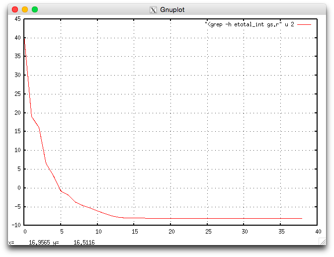
Fig. 1 Intermediate energy <etotal_int> during self-consistent iterations.
This allows for a quick inspection of the convergence of the calculation.
Note
The gnuplot program is not provided with Qbox and must be installed separately.
Larger XML fragments such as the <atomset> element can be extracted from
output files using xml_grep:
$ xml_grep atomset gs.r

 <?xml version="1.0" ?>
 <xml_grep version="0.9" date="Thu Jul 26 15:42:21 2018">
 <file filename="gs.r">
   <atomset>
     <unit_cell a=" 15.00000000   0.00000000   0.00000000" b="  0.00000000  15.00000000   0.00000000" c="  0.00000000   0.00000000  15.00000000"/>
     <atom name="C" species="carbon">
       <position> 0.00000000 0.00000000 0.00000000 </position>
       <velocity> 0.00000000 0.00000000 0.00000000 </velocity>
       <force> -0.00000095 -0.00000463 -0.00000191 </force>
     </atom>
     <atom name="H1" species="hydrogen">
       <position> 1.25000000 1.25000000 1.25000000 </position>
       <velocity> 0.00000000 0.00000000 0.00000000 </velocity>
       <force> -0.01459937 -0.01459776 -0.01459803 </force>
     </atom>
     <atom name="H2" species="hydrogen">
       <position> 1.25000000 -1.25000000 -1.25000000 </position>
       <velocity> 0.00000000 0.00000000 0.00000000 </velocity>
       <force> -0.01460360 0.01460308 0.01460326 </force>
     </atom>
     <atom name="H3" species="hydrogen">
       <position> -1.25000000 1.25000000 -1.25000000 </position>
       <velocity> 0.00000000 0.00000000 0.00000000 </velocity>
       <force> 0.01460679 -0.01460536 0.01460398 </force>
     </atom>
     <atom name="H4" species="hydrogen">
       <position> -1.25000000 -1.25000000 1.25000000 </position>
       <velocity> 0.00000000 0.00000000 0.00000000 </velocity>
       <force> 0.01460517 0.01460393 -0.01460412 </force>
     </atom>
   </atomset>
 </file>
 </xml_grep>
The above calculation of the electronic ground state used approximate atomic coordinates based on a reasonable guess of the structure of the CH4 molecule. A natural next step is to optimize the molecule geometry to find its minimum energy structure.
Geometry optimization
The complete input file for the geometry optimization of CH4 is:
1# CH4 structure optimization
2load gs.xml
3set wf_dyn PSDA
4set xc PBE
5set scf_tol 1.e-8
6set atoms_dyn CG
7run 10 10
8save cg.xml
We now analyze in detail the input script:
In line 2, the load command reads the description of the sample previously saved in the file
gs.xmlat the end of the ground state calculation.Lines 3-5 set the wf_dyn, xc, and scf_tol variables as in the ground state calculation.
Line 6 selects the algorithm used to move atoms as CG for “conjugate gradient).
Line 7 invokes the run command to perform the calculation, with 10 ionic steps (where atoms are moved) and 10 self-consistent iterations before each move of the atoms.
Line 8 uses the save command to write the description of the sample to the file
cg.xmlfor later use in another calculation.
The evolution of the energy during the geometry optimization can be visualized
using the etotal.plt script:
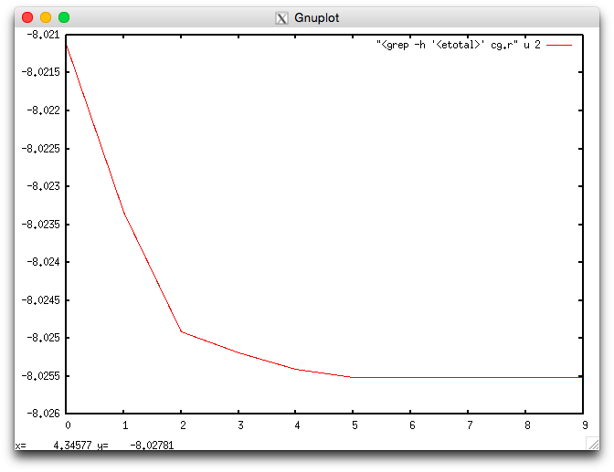
Fig. 2 Energy <etotal> during the geometry optimization.
Numerical values of <etotal> can be extracted using xml_grep:
$ xml_grep etotal cg.r
<?xml version="1.0" ?>
<xml_grep version="0.9" date="Fri Jul 27 16:58:40 2018">
<file filename="cg.r">
  <etotal>      -8.02111902 </etotal>
  <etotal>      -8.02333130 </etotal>
  <etotal>      -8.02491158 </etotal>
  <etotal>      -8.02519366 </etotal>
  <etotal>      -8.02540308 </etotal>
  <etotal>      -8.02550918 </etotal>
  <etotal>      -8.02550995 </etotal>
  <etotal>      -8.02551261 </etotal>
  <etotal>      -8.02551265 </etotal>
  <etotal>      -8.02551269 </etotal>
</file>
</xml_grep>
Molecular dynamics
We now demonstrate the use of Qbox in a short Born-Oppenheimer molecular dynamics simulation. The simulation consists of 100 MD steps, with a time step of 10 (a.u.). Atomic velocities are initialized with random values from a Maxwell-Boltzmann distribution at a temperature of 400 K.
The complete input file for the molecular dynamics simulation of CH4 is:
 1# CH4 molecular dynamics simulation
 2load cg.xml
 3set wf_dyn PSDA
 4set xc PBE
 5set scf_tol 1.e-6
 6set dt 10
 7set atoms_dyn MD
 8randomize_v 400
 9run 100 10
10save md.xml
We now analyze in detail the input script:
In line 2, the load command reads the description of the sample previously saved in the file
cg.xmlat the end of the geometry optimization.Lines 3-5 set the wf_dyn, xc, and scf_tol variables as in the ground state and geometry optimization calculations.
Line 6 sets the variable dt (time step) to 10 (a.u.). 1 (a.u.) = 0.02418885 fs.
Line 7 selects the algorithm used to move atoms as MD (molecular dynamics).
Line 8 uses the randomize_v command to initialize atomic velocities with random numbers drawn from a Maxwell-Boltzmann distribution at T=400 K.
Line 9 invokes the run command to perform the calculation. The simulation consists of 100 ionic steps, with 10 self-consistent iterations before each step.
Line 10 uses the save command to write the description of the sample to the file
md.xmlfor later use in another calculation.
The evolution of the energy during the simulation can be visualized using
the etotal.plt script:
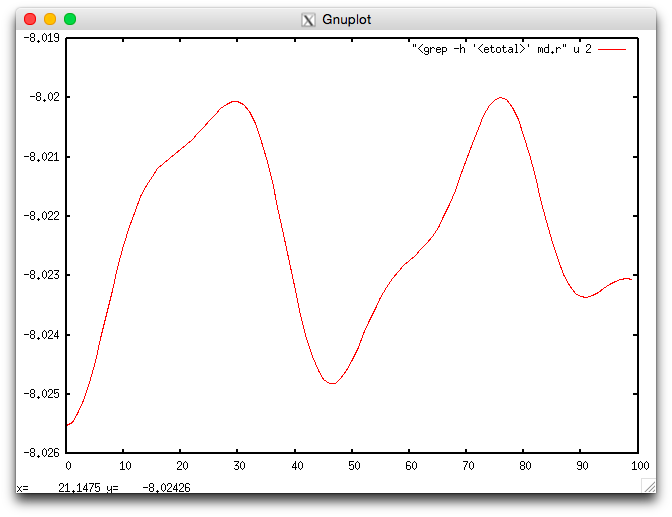
Fig. 3 Energy <etotal> during the molecular dynamics simulation.
The quality of the simulation can be monitored by visualizing the energy
together with the constant of the motion (element <econst>):
\[E_{\rm const} = E_{\rm KS} + T_{\rm ion}\]
where \(E_{\rm KS}\) is the (Kohn-Sham) energy, represented by the value
of the element <etotal> and \(T_{\rm ion}\) is the kinetic energy
of the ions. The script econste.plt shows the value of both <etotal>
and <econst>:
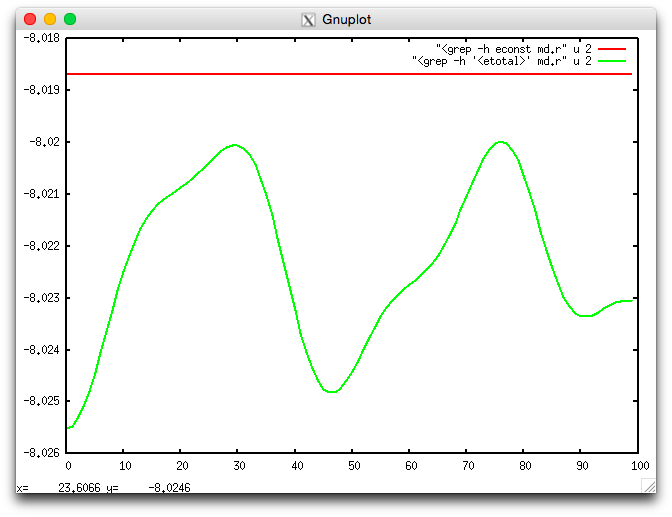
Fig. 4 Energy <etotal> and constant of the motion <econst> during the MD simulation.
The quantity <econst> shows no appreciable variation on the scale of the
variation of <etotal>, confirming the validity of the approximations
used in the simulation. Inaccurate calculations of the electronic ground
state between MD steps (due e.g. to an insufficient number of self-consistent
iterations) typically lead to a sizeable drift in the value of <econst>.
Similarly, oscillations in <econst> may be observed if the value of the
time step dt is too large.
The atomic trajectories can be visualized by generating an “xyz” file
containing the atomic positions at each step of the simulation, and using
a visualization program such as VMD. The xyz file can be generated using the
qbox_xyz.py script:
$ qbox_xyz.py md.r > md.xyz
Rendering the file md.xyz with VMD allows for visual inspection of the
trajectories using the VMD graphical user interface:
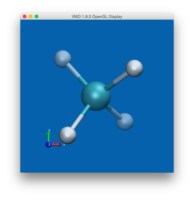
Fig. 5 Visualization of the CH4 molecule using the VMD program.